Data Tables
Estimated Bird Abundance
Estimated abundance for each bird species was calculated by summing bird species abundance at each secondary sampling unit (SSU). Bird species are identified with a unique four-digit code (e.g.: AMPI represents American Pipit). Secondary sampling units are identified with a three-letter code denoting mountain, a one-letter code denoting bioclimate zone (S = subalpine, T = alpine tundra), and a one-digit code denoting the SSU within that bioclimate zone (e.g.: AND_S1 represents subalpine site 1 on Mount Anderson) (Figure 10). There were a total of 71 sample sites and 42 bird species.
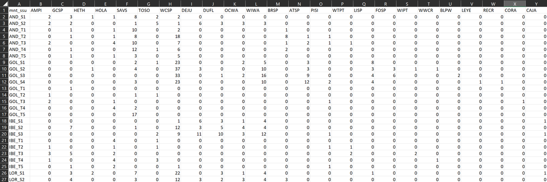
Figure 10: Sample of bird abundance data used in visualization and analysis.
Shrub Dominance Elements
Shrub height was calculated for each secondary sampling unit by averaging the heights of all shrubs sampled at each SSU (Figure 11).
Shrub density was calculated for each secondary sampling unit using the Point Centered Quarter Method (PCQM). Distances to the nearest shrub in each height category were averaged, and 1 m was added to all average distances to avoid asymptotically high values when distances to shrubs were low. Shrub density per 100 m^2 was calculated using: 100/(d^2), where d is the average distance to the nearest shrub at each site. Average distance was removed from data frame prior to visualization and analysis.
Shrub stem count was calculated for each secondary sampling unit by averaging the stem counts of all shrubs sampled at each SSU.

Figure 11: Sample of shrub dominance elements table used in data visualization and analysis.
Shrub Species
Shrub species at each secondary sampling unit were calculated by summing the number of each shrub species sampled at each SSU. A total of 19 different species were identified. Two groups were identified only to Genus level (Alnus spp and Salix spp) due to the high number of species in each genus. NA column was removed prior to visualization and analysis (Figure 12).
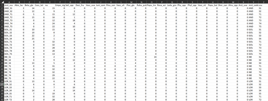
Figure 12: Sample of shrub species table used in data visualization and analysis.
Data Visualization
Bird Abundance
|
The bird data was visualized using an NMDS to assess associations between bird species and the bioclimate zones. There were three species strongly associated with alpine habitat: (1) Horned Lark (HOLA), (2) White-tailed Ptarmigan (WTPT), (3) American Pipit (AMPI), and (4) Surfbird (SURF) (Figure 13). The species strongly associated with the subalpine include: (1) White-crowned sparrow (WCSP), (2) Wilson's Warbler (WIWA), (3) Orange-crowned Warbler, (4) Dusky Flycatcher (DUFL), and (5) Dark-eyed Junco (DEJU)) (Figure 13). |
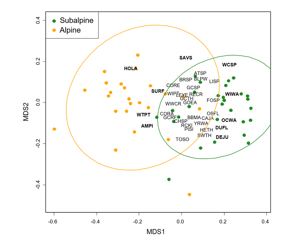
Figure 13: NMDS ordination representing bird species associations with bioclimate zone. Green and orange points and ellipses represent sampling sites in the subalpine and alpine habitats respectively. Bird species are identified by a unique four-letter code. Bird species in bold are highly associated with the corresponding bioclimate zone. Vectors were removed to make the plot easier to read, but bird code location corresponds to the end of each vector.
|
Shrub Dominance
|
The shrub dominance data was also visualized using an NMDS. Shrub height appears to be a strong driver of distinguishing between the subalpine and alpine habitats as seen by the general horizontal nature of the points that fall along the same axis as the height vector (Figure 14). Shrub density and stem count appear to be negatively associated with each other based on the vectors facing in nearly opposite directions (Figure 14). While not intuitive, this association does make sense based on my sampling method. Stem count was based on the number of stems per plant, but density was based on plants as a whole. Therefore, if a shrub has more stems and takes up more horizontal space, the distance between each shrub would be greater and would result in a lower density based on my calculation method. |
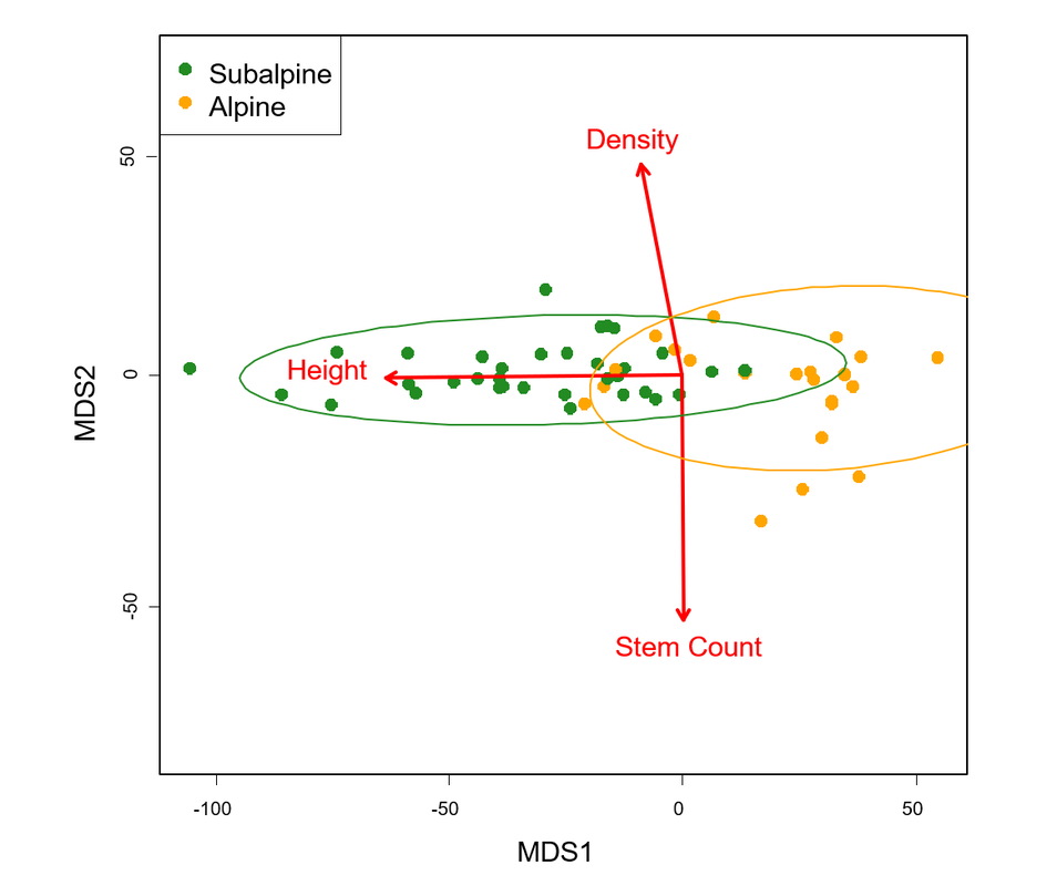
Figure 14: NMDS ordination representing shrub dominance associations with bioclimate zone. Green and orange points and ellipses represent sampling sites in the subalpine and alpine habitats respectively.
|
